Fiber Weave Skew Modeling: Analytical Bounds and Statistical Skew Prediction

Fiber weave skew cannot be predicted as a single number for a given board. Registration tolerance and weave non-uniformity mean the position of a trace relative to the glass bundles is set by chance during fabrication, so skew is a statistical distribution rather than a fixed offset. Two modeling approaches address this: an analytical method that bounds the minimum and maximum dielectric constant a fabrication process can produce, and a statistical method that predicts the probability of exceeding a given skew limit for a specific glass weave style.

The previous article in this series discussed how the fiber-weave effect can introduce intra-pair skew in differential signaling, ultimately leading to eye diagram closure. Building on that foundation, this second part addresses an important aspect of the problem: fiber weave skew (FWS) is inherently random and requires complex modeling to capture its effects accurately. To gain insight into the characteristics of FWS, we examine two distinct approaches for modeling this phenomenon. The first uses simple analytical formulas to estimate the bounds of dielectric constant variation, while the second introduces a modeling framework that enables statistical skew prediction. Before delving into the modeling approaches, it’s worth understanding what makes FWS inherently random in the first place.

Why Is Fiber Weave Skew Random?

Because trace-to-weave alignment is set by chance during fabrication. Registration tolerance introduces an uncontrollable offset between the copper artwork and the glass weave beneath it, and the weave itself is non-uniform. Two boards built from identical Gerber data on identical laminate can therefore exhibit different skew.

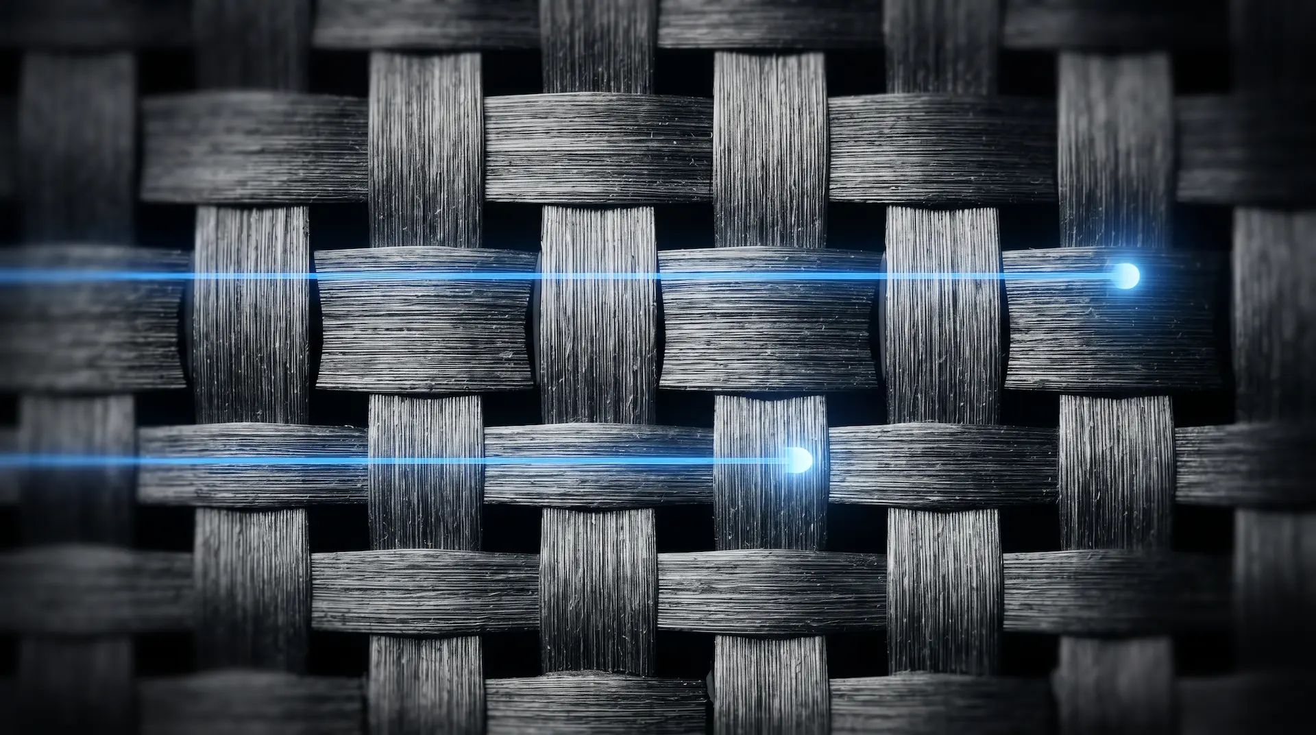
The random nature of FWS stems largely from manufacturing variations that are unavoidable in PCB fabrication. Even when a fabricator uses identical Gerber data and the same laminate materials for a batch of 100 boards, trace-to-weave alignment will still vary randomly from board to board. A key contributor is registration tolerance—the small, uncontrollable offset between the copper artwork and the underlying glass weave. As a result, Board #1 may pass high-speed testing without issue, while Board #2 fails due to excessive FWS. Weave non-uniformity also plays a role: during weaving, glass bundles bunch, stretch, and twist, creating an irregular dielectric landscape, as shown in Figure 1.

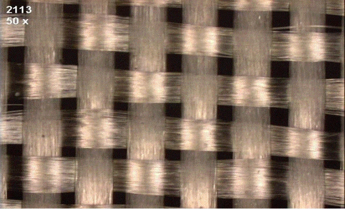
Engineers cannot predict or control exactly where a trace lands relative to the fiberglass weave, turning FWS into a statistical outcome. One cannot simply declare that a board will exhibit a skew of exactly X ps/in.

FWS modeling can be approached in different ways. Some methods focus on worst-case skew; others provide a statistical framework for skew prediction. The first approach examined here, proposed by Bert Simonovich, uses simple equations to bound the dielectric constant (Dk) and estimate the worst-case skew.

How Do You Bound Dk Variation? Simonovich’s Analytical Method

By using two extreme glass cloth styles as statistical proxies. The loose, resin-rich 106 style sets the low-Dk bound and the tight, glass-rich 7628 style sets the high-Dk bound. Combining their 3-sigma tolerances gives a Dkmin and Dkmax pair that can be assigned to opposite legs of a differential pair to simulate worst-case skew.

Instead of modeling the precise fiber-weave geometry beneath a differential pair, this method provides simple equations that estimate the minimum and maximum Dk values for use in differential pair simulation.

To estimate these Dk extremes, the method uses dielectric data from the 106 and 7628 fiberglass cloth styles as statistical proxies. The 106 style, with its loose weave and high resin content, represents the low-Dk extreme. The 7628 style, with its tight weave and high glass content, represents the high-Dk extreme. Both are illustrated in Figure 2.

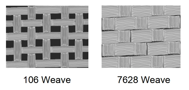
It’s important to note that these two cloth styles may not actually be used in a given board design. They serve only to bracket the range of Dk variation a fabricator's process can produce. Let’s see how the dielectric data from these two laminates can be used to estimate bounds on Dk.

Deriving Dkmin and Dkmax from Material Data

Table 1 shows the dielectric values reported by Park Nelco for the 106 and 7628 cloth styles in its N4000-13 material system.

Table 1: Dielectric values for Park Nelco’s 106 and 7628 cloth styles. (Source: Simonovich 2011, courtesy of Bert Simonovich.)

For each cloth style, the Dk can be viewed as a random variable with a known mean and standard deviation. For example, the mean of the 7628 cloth is given by:

Applying basic statistics, the standard deviation for this weave pattern is:

For the 106 cloth style, the four Dk values yield a mean of Dkavg_106=3.34 and a standard deviation of 𝜎106=0.13. Applying the same calculation to the 7628 style gives Dkavg_7628=3.97 and 𝜎7628=0.09.

Recall that timing skew in a differential pair arises from differences in the dielectric constant seen by each trace. Since the statistical variation in local Dk is represented by the extremes of the 106 and 7628 weave styles, we’re primarily interested in the Dk contrast between these two materials. For this reason, we define ΔDk as the difference between their dielectric constants:

The mean of ΔDk is simply the difference between the mean Dk values of the two weave styles:

The maximum ΔDk is found by combining the relative 3-sigma tolerances of both weaves, each expressed as a fraction of that weave’s mean Dk, via a root-sum-square (RSS) approach. Scaling that result by ΔDkavg and adding it to ΔDkavg gives:

From these values, a tolerance factor Tol is established:

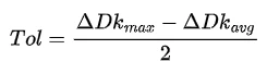
Applying Tol symmetrically gives the localized Dkmin and Dkmax bounds:

and

Noting that the difference between ΔDkmax and ΔDkavg represents the one-sided 3-sigma spread of the ΔDk distribution, one might ask why the tolerance factor Tol is defined as half of that spread. The reason is that ΔDk captures the Dk difference between the two traces, not the variation of each trace individually. To distribute the variation symmetrically, the mean Dk of the 106 style is shifted downward by half the 3-sigma spread, while the mean of the 7628 style is shifted upward by the same amount.

By establishing these distinct boundaries, designers can assign Dkmin to one leg of a differential pair and Dkmax to the other within an EDA tool (such as Agilent ADS) and determine the worst-case timing skew.

Worked Example: Calculated Dk Bounds vs. MATLAB Simulation

The whitepaper that introduces this method includes a numerical example based on the data in Table 1. We reproduce that example here and compare its calculated bounds with a MATLAB simulation. From Table 1, the relevant values are:

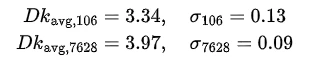
Given these values, we wish to estimate the bounds on Dk.

Solution:

The average Dk difference between the two weave styles is:

The maximum of ΔDk is obtained as:

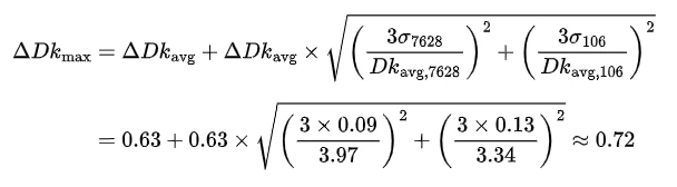
This corresponds to a tolerance factor of Tol=(0.72-0.63)/2≈0.05, yielding the following Dk bounds:

and

As a verification step, we modeled the two weave styles as independent normal random variables with the same means and standard deviations in MATLAB. Using 10,000 samples for each weave style, we obtain the histogram of 20,000 combined samples, as shown in Figure 3.

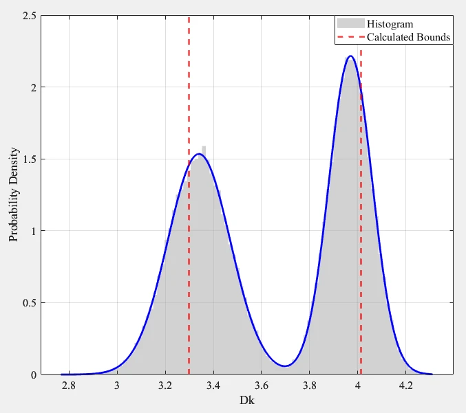
The two peaks reflect the underlying normal distributions: the right peak captures the Dk variation of the 7628 style, and the left peak captures that of the 106 style. The red dashed lines indicate the calculated Dk bounds of 3.29 and 4.02 obtained from the analysis. The simulated data, however, extends beyond these limits.

The above simulation yields only one realization of the extreme values. To obtain a more reliable comparison, the simulation was repeated 100 times, and for each trial the minimum and maximum Dk values were recorded. Figure 4 shows the distribution of these minima and maxima, alongside the calculated bounds.

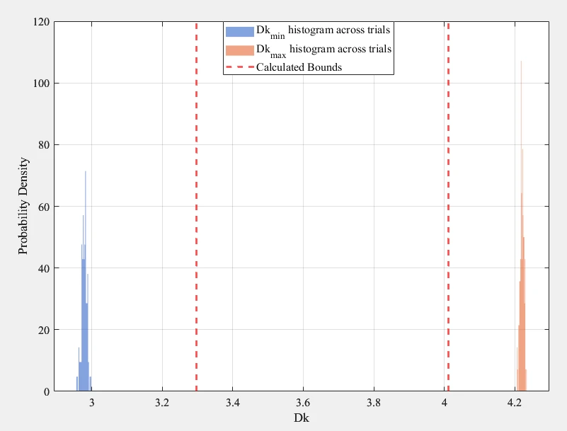
Rather than taking the absolute minimum and maximum of each trial, which are sensitive to sample size and outliers, the bounds shown in Figure 4 were computed using a quantile-based approach. Specifically, the 0.135th and 99.865th percentiles were extracted from the 20,000 combined samples in each trial. These percentiles correspond to the ±3σ tail probabilities used in the analytical method, making the comparison conceptually consistent.

As seen in Figure 4, the histogram of per-trial Dk minima sits slightly below the calculated lower bound, while the histogram of maxima lies a little above the calculated upper bound. This indicates that although the analytical method provides a useful hand-calculation for estimating Dk bounds, the simulated bounds are somewhat wider than those predicted by the equations.

While this analytical method offers a quick estimate of the Dk range, it doesn’t provide information about the likelihood of the Dk extremes. This leads us to the second approach covered in this article, which can analyze FWS for yield estimation.

How Do You Predict Fiber Weave Skew Statistically?

By sweeping a trace across one full period of the weave in electromagnetic simulation, extracting the delay at each offset, and treating that offset as a uniformly distributed random variable. The resulting distribution yields the probability that delay or skew exceeds a chosen limit, which converts a weave style choice into a yield estimate.

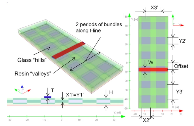
In "Quantification of Delay and Skew Uncertainty due to Fiber Weave Effect in PCB Interconnects," Manukovsky, Shlepnev, and Mordooch propose a method for predicting FWS statistically. The approach models the weave as an idealized geometry of rectangular glass-rich and resin-rich regions with sharp boundaries, as shown in Figure 5.

The trace offset relative to the weave pattern is swept across one full period of the weave, and the delay at each position is extracted from EM simulation. This offset is treated as a random variable with a uniform distribution. Figure 6 shows delay as a function of trace offset for four different weave styles.

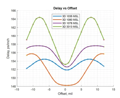
As observed, the delay variation with offset resembles a sinusoidal function. This is a natural consequence of sweeping the trace across the periodic glass-resin pattern. Using the resulting delay‑versus‑offset curve, the statistical distribution of delay deviation is computed and plotted as a histogram for each weave style, as shown in Figure 7.

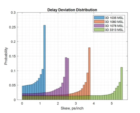
The largest delay deviations occur when the trace sits directly over a glass bundle or a resin-rich region. Mid-range deviations arise in the transitional zones between these two extremes, where the effective permittivity is near its average. Because the trace spends more time over the glass-rich and resin-rich regions than in the transitions, the resulting histogram of delay deviation is U-shaped: values near the minimum and maximum are the most probable, while those near the average are the least.

To turn these observations into a practical measure of uncertainty, the complementary cumulative distribution function (CCDF) of the delay deviation is computed. The CCDF, shown in Figure 8, gives the probability that the delay deviation exceeds a specified value.

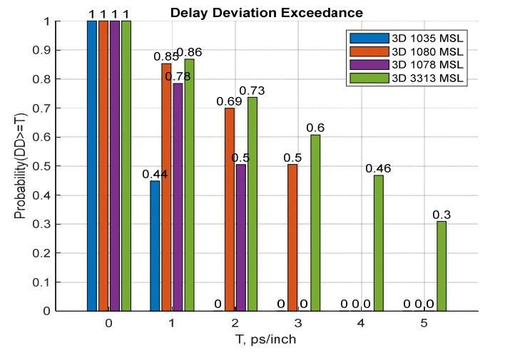
The authors introduce a specific metric, called Delay Deviation Exceedance (DDE), which expresses the probability that the delay deviation exceeds a specified limit. As an example, consider a DDR design that requires the delay uncertainty to remain below 3 ps/inch. The 1080 and 3313 weave styles would not meet that requirement. With those fabrics, the likelihood of exceeding 3 ps/inch is roughly 50% for 1080 and 61% for 3313, giving engineers a practical estimate of the expected yield in mass‑production boards.

A similar procedure is applied in the paper to evaluate the intra-pair skew uncertainty in differential signaling. The authors compute the differential skew exceedance (DSE), which gives the probability that the differential skew exceeds a specified limit. The resulting DSE probabilities for the examined weave styles are shown in Figure 9.

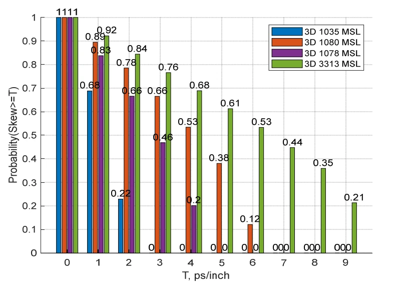
For example, the DSE data show that a skew limit of 3 ps/inch would only be met by the 1035 weave style, whereas the probability of exceeding this limit is about 47% for 1078, 67% for 1080, and 77% for 3313.

Probabilities that delay deviation (DDE) or intra-pair skew (DSE) exceeds 3 ps/inch, for the trace geometry examined in the source paper. Source: Manukovsky et al. 2023.

Limitations and Practical Considerations

Any FWS model carries assumptions worth noting. In the present work, for example, the weave is idealized with sharp boundaries between glass-rich and resin-rich regions, whereas real laminates exhibit more gradual transitions.

Furthermore, the results are geometry-dependent. A different trace width or line separation can produce different delay and skew variation, so each design should derive its own DDE and DSE curves from EM simulations or measurements based on the intended trace geometry.

Another limitation of the analysis is that it only considers traces running parallel to the glass bundles; traces routed at an angle can interact with the weave differently and may exhibit a distinct pattern of delay and skew variation.

Conclusion

Numerous modeling approaches exist for FWS, each with its own strengths and limitations — the two examined here are just representative examples. The analytical method gives a fast hand-calculation for the Dk range but says nothing about how likely the extremes are. The statistical method costs more effort and returns something the first cannot: a probability, and with it a yield estimate. Understanding such methods allows engineers to proactively explore the design space, establish safe trace length budgets, and determine whether mitigation techniques like transmit de-emphasis or angled routing are needed before committing to fabrication. Equally important is the ability to estimate the expected yield in the presence of FWS, which helps balance performance targets against manufacturing realities.

Related Reading

Part 1: Understanding Fiber Weave Effect: From Glass Weave to Differential Skew

Part 2: Fiber Weave Skew Modeling (this article)

Part 3: Mitigating Fiber Weave Skew, from Spread Glass to Routing Angle (coming soon)

Frequently Asked Questions

Why is fiber weave skew random?

Trace-to-weave alignment is set by chance during fabrication. Registration tolerance introduces a small, uncontrollable offset between the copper artwork and the glass weave beneath it, and the weave itself is non-uniform because glass bundles bunch, stretch, and twist during weaving. A fabricator can build 100 boards from identical Gerber data on identical laminate and each one will have a slightly different trace-to-weave relationship. One board may pass high-speed testing while the next fails.

Can fiber weave skew be predicted exactly for a given board?

No. Because the trace position relative to the weave is random, skew is a statistical distribution rather than a fixed value. You cannot declare that a board will exhibit exactly X ps/inch of skew. What you can do is bound the range analytically, or compute the probability of exceeding a chosen limit and treat that as a yield estimate.

How do you estimate worst-case Dk variation from the fiber weave?

Simonovich's analytical method uses two extreme glass cloth styles as statistical proxies: the loose, resin-rich 106 style for the low-Dk bound and the tight, glass-rich 7628 style for the high-Dk bound. The relative 3-sigma tolerances of both styles are combined via root-sum-square, scaled by the mean Dk difference, halved to give a tolerance factor, and applied symmetrically around each style's mean. In the worked example this yields bounds of Dkmin = 3.29 and Dkmax = 4.02, which can be assigned to opposite legs of a differential pair in an EDA tool to simulate worst-case skew.

What are DDE and DSE?

Delay Deviation Exceedance (DDE) is the probability that the propagation delay deviation on a single-ended trace exceeds a specified limit. Differential Skew Exceedance (DSE) is the equivalent for intra-pair skew on a differential pair. Both are derived from the complementary cumulative distribution function of delay computed by sweeping a trace across one period of the weave in electromagnetic simulation. They convert a weave style choice into a quantified probability of failure.

Which glass weave styles are worst for fiber weave skew?

Of the four styles examined in the source paper at a 3 ps/inch limit, 3313 is the worst, with a 77% probability of exceeding that differential skew limit, followed by 1080 at 67% and 1078 at 47%. Only 1035 clears the limit outright at 0%. These figures are specific to the trace geometry modeled in the paper, so a different trace width or pair separation will shift them.

Why do the analytical and simulated Dk bounds disagree?

They agree in concept and differ in width. When the two weave styles are modeled as independent normal random variables and sampled 20,000 times per trial across 100 trials, the simulated minima sit slightly below the calculated lower bound and the maxima slightly above the upper bound. The analytical equations remain a useful hand-calculation, but they are marginally optimistic about how far the extremes reach.

References:

Simonovich, Lambert. 2011. “Practical Fiber Weave Effect Modeling.” White Paper, Issue 2. LAMSIM Enterprises Inc., January 10. http://www.lamsimenterprises.com/Practical_Fiber_Weave_Modeling_Iss2_Jan10-11.pdf.

Manukovsky, Alex, Yuriy Shlepnev, and Shimon Mordooch. 2023. “Quantification of Delay and Skew Uncertainty due to Fiber Weave Effect in PCB Interconnects.” Paper presented at the 2023 IEEE 32nd Conference on Electrical Performance of Electronic Packaging and Systems (EPEPS), Milpitas, CA, USA, October 15-18. https://www.simberian.com/AppNotes/FWE_Quantification_EPEPS_2023_final.pdf.