Via Stubs in PCB Design: Resonance, Insertion Loss Nulls, and Back Drilling

Key Takeaways

A via stub is the unused portion of a plated through-hole via barrel that extends past the layer where the signal transitions to a routing trace. It behaves as an open-circuited transmission line, and at the frequency where its length equals a quarter wavelength, the reflected wave cancels the signal and creates a deep null in insertion loss. Two rules of thumb set the maximum stub length for a target data rate: the 7th harmonic criterion and Bogatin’s rule. Both put the limit at roughly 5 to 6 mils for a 112G PAM4 link. Stubs also hide in connector pads, edge-finger wipes, and press-fit pins, and back drilling is the standard way to shorten via stubs on 30+ Gbps channels.

• Stub length sets the resonant frequency. A 100-mil stub with an effective Dk of 6.16 resonates at about 11.9 GHz. A 270-mil backplane stub puts its first null near 4.4 GHz, close enough to the 5 GHz Nyquist frequency to close the eye of a 10 Gbps NRZ signal.
• Use the effective Dk of the via structure, not the datasheet Dk. Excess capacitance between the barrel and the plane layers raises the effective Dk (6.16 versus a published 3.65 in this example). The published value predicts a resonant frequency higher than the one observed in hardware.
• Both rules of thumb agree at 112G PAM4. Using the 56 GBd symbol rate rather than the 112 Gbps bit rate, the 7th harmonic criterion gives a maximum stub length of 6 mils and Bogatin’s rule gives 5.3 mils.
• Hidden stubs need an audit too. A connector landing pad entered from the wrong side, the copper left past an edge-finger wipe, and a press-fit pin on an upper or middle layer all act as unterminated stubs at high data rates.
• Back drilling is the standard fix for via stubs. It re-drills the via from the opposite side to remove the unused barrel, bringing stubs down to the 5 to 10 mil range that 30+ Gbps channels demand, at added manufacturing cost. Part 2 of this series covers it in detail.

At multi-gigabit data rates, even minor geometric structures like via stubs can compromise signal integrity. A via stub is the unused, open-circuited portion of a plated through-hole barrel that extends past the target layer where the signal transitions to a routing trace. This parasitic structure acts as an unterminated transmission line, causing problems by reflecting electrical energy back into the main channel; at resonant frequencies, these reflections create destructive interference that introduces insertion loss nulls and collapses the eye diagram. This article examines the physics of stub-induced resonance, presents two industry rules of thumb for calculating maximum allowable stub length, and highlights the "hidden stubs" found in component pads and connector features that layout engineers frequently miss. It concludes by introducing back drilling, the standard manufacturing remedy that Part 2 of this series will examine in detail.

The Physics: Why Via Stubs Are High-Speed Killers

A through-hole via that drops a signal onto an inner layer leaves a dangling metallic cylinder below the transition point.

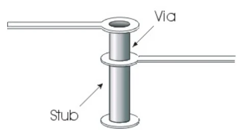
In high-speed design, this via stub acts as an open-circuited transmission line. When a signal reaches the stub junction, part of the energy continues along the intended trace, while the remainder travels down the stub, hits the open circuit, and bounces back, as illustrated in Figure 2.

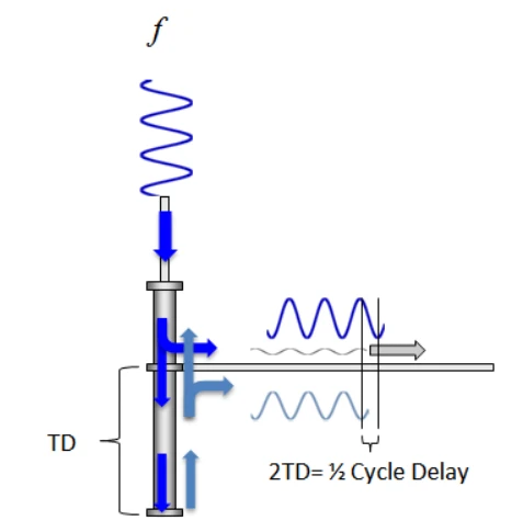
The figure above shows the scenario where a quarter-wavelength stub causes the reflected signal (shown in light blue) to accumulate a 180-degree phase shift by the time it arrives back at the junction. Consequently, this out-of-phase reflection destructively interferes with the primary signal (shown in blue) on the intended path, effectively canceling it out.

Specifically, the signal portion traveling down the stub accumulates a 90-degree phase shift over that quarter-wavelength distance (L_stub=λ/4). At the open-circuited end, the infinite impedance boundary causes a 100% in-phase voltage reflection. Traveling back through the stub adds another 90-degree shift, meaning the reflected wave returns to the junction exactly 180 degrees out of phase with the primary signal. This perfect phase opposition causes complete destructive interference, creating a deep notch filter in the insertion loss spectrum. The left plot in Figure 3 shows the simulated insertion loss response of a backplane channel with a long 270-mil stub, while the right diagram shows the corresponding data eye for a 10 Gbps, non-return-to-zero (NRZ) signal.

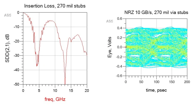
The long stub introduces quarter-wave resonant nulls at approximately 4.4 GHz and its subsequent odd harmonics (with the third harmonic visible at 13.2 GHz). Because the fundamental null occurs near the 5 GHz Nyquist frequency of the 10 Gbps signal, the data eye closes completely.

Calculating Via Stub Resonant Frequency from Stub Length

Engineers need to estimate where the resonant frequency falls to determine whether a stub length threatens the target data rate. To illustrate this calculation, consider a high-speed channel in a thick PCB stackup where a layer transition creates a 100-mil (2.54 mm) via stub surrounded by an effective dielectric constant of Dk_eff=6.16.

To determine the resonant frequency, the signal propagation velocity v within the PCB must first be calculated. Signals slow down relative to the speed of light in a vacuum (c=3×10⁸ m/s) based on the effective dielectric constant of the surrounding material, as defined by the following relationship:

\[ v = \frac{c}{\sqrt{Dk_{eff}}} = \frac{3 \times 10^{8}\ \text{m/s}}{\sqrt{6.16}} \approx 1.21 \times 10^{8}\ \text{m/s} \]

Equation 1

Destructive cancellation occurs when the physical length of the stub L_stub equals one-quarter of the signal's wavelength 𝜆/4. Therefore, the wavelength at the resonant frequency is:

\[ \lambda = 4 \times L_{stub} = 4 \times 2.54\ \text{mm} = 10.16\ \text{mm} = 0.4\ \text{inches} \]

Equation 2

With the signal velocity and wavelength determined, the resonant frequency can be found using the following relationship:

\[ f = \frac{v}{\lambda} = \frac{1.21 \times 10^{8}\ \text{m/s}}{10.16 \times 10^{-3}\ \text{m}} \approx 11.91\ \text{GHz} \]

Equation 3

At this specific frequency, the destructive resonant notch occurs, heavily attenuating the transmitted signal. While 11.91 GHz represents the absolute zero-power null where the signal is completely canceled, significant degradation occurs much earlier due to the wide roll-off of the stub's notch filter (see Figure 3). Estimating where this attenuation becomes critical requires evaluating a primary benchmark, namely the 7th harmonic criterion (Simonovich 2017).

Translating Stub Length to Target Data Rates: The 7th Harmonic Criterion

The resonant frequency itself is not the primary metric a designer needs; rather, the goal is determining whether the channel can support the target data rate. Because a via stub’s true 3-dB bandwidth requires full-wave electromagnetic (EM) simulation to quantify, engineers rely on the 7th harmonic criterion as a practical rule of thumb. This guideline dictates that the first resonant null must fall at or past the 7th harmonic of the Nyquist frequency. Doing so pushes the notch filter's wide attenuation skirt far enough out to preserve the critical 5th harmonic responsible for signal rise time.

Following the same procedure used in the numerical example, combining Equations 1 through 3 establishes a general relationship for the resonant frequency:

\[ f_o = \frac{c}{4 \times L_{\text{stub}} \times \sqrt{Dk_{\text{eff}}}} \]

Equation 4

By defining the speed of light c as 11.8 in/ns and the stub length L_stub in inches, the formula evaluates the resonant frequency f_o in GHz. Equating the resonant frequency with seven times the Nyquist frequency yields:

\[ f_o = 7 \times f_{\text{Nyquist}} \]

Equation 5

The Nyquist frequency is half the baud rate, producing:

\[ f_o = 7 \times \left(\frac{\text{Baud}}{2}\right) = 3.5 \times \text{Baud} \]

Equation 6

Equating Equations 4 and 6 yields an expression for L_stub:

\[ L_{\text{stub}} = \frac{0.84}{\text{Baud} \times \sqrt{Dk_{\text{eff}}}} \]

Equation 7

The unit for Baud in this equation is gigabaud (GBd), or gigasymbols per second. To put these concepts into perspective, consider a 112G four-level pulse amplitude modulation (PAM4) link. Because each symbol carries two bits, the 112 Gbps data rate requires a symbol rate of 56 GBd, which establishes a 28 GHz Nyquist frequency. Assuming Dk_eff=6.16, Equation 7 yields:

\[ L_{\text{stub}} = \frac{0.84}{56 \times \sqrt{6.16}} = 0.0060\ \textit{inches} = 6\ \textit{mils} \]

Equation 8

This value defines the maximum allowable stub length required to isolate the signal from the destructive effects of the quarter-wave resonant null. For traditional through-hole vias, achieving a remaining stub of roughly 6 mils pushes advanced PCB fabrication to its physical limits. Standard commercial manufacturing tolerances often leave a stub in the range of 5 to 10 mils, demonstrating that adhering to the 7th harmonic criterion poses a substantial challenge at 112G PAM4 and beyond.

Key Considerations for the 7th Harmonic Criterion

The 7th harmonic criterion involves several nuanced principles; breaking down these core concepts provides a much more intuitive understanding of the overall method.

What Is the Nyquist Frequency?

The method equates the resonant frequency with seven times the Nyquist frequency. In high-speed digital communications, the Nyquist frequency is defined as half the symbol rate (the baud rate). Derived from Nyquist's pulse-shaping theorem, it represents the minimum bandwidth required to transmit independent pulses at a given rate without introducing intersymbol interference (ISI). While the actual power spectrum of a digital signal extends far beyond this frequency due to the high-frequency content of sharp pulse transitions, the Nyquist frequency serves as a useful metric for analyzing the bandwidth requirements of high-speed links.

Why the 7th Harmonic?

The "7th harmonic" rule of thumb for via stub resonant nulls is not a fundamental physical law but a practical signal-integrity margin designed to preserve the signal's rise-time behavior. Digital signal energy extends well beyond the Nyquist frequency, and preserving the steep rising and falling edges requires keeping frequency components up to roughly five times the Nyquist frequency intact (Bogatin 2014a). Because a via stub produces a resonant null that repeats at odd harmonics, positioning the first null at or above the 7th harmonic keeps the notch safely above that critical 5th-harmonic band. If those higher frequencies are attenuated, the edges become sluggish and the eye diagram closes.

Why Does Effective Dk Exceed Published Values?

The effective dielectric constant of the via structure Dk_eff is typically higher than the material's bulk Dk due to excess capacitance between the via barrel and the plane layers it passes through (for example, 6.16 versus a published Dk of 3.65). Laminate datasheets typically publish bulk Dk values measured along the z-axis (thickness direction) rather than the effective Dk that a vertical via structure experiences in the x-y plane. A vertical via is a complex 3D structure in which small anti-pad clearances concentrate the electric field between the barrel and plane layers, so the via stores more charge per unit length than an equivalent transmission line and exhibits a higher effective dielectric constant. This increased value slows signal propagation down the stub, shifting the destructive resonant null to a lower, more dangerous frequency. Consequently, if one uses the standard published Dk in the stub-length formula, the predicted resonant frequency will be higher than what is actually observed in hardware (see Equation 4).

Bogatin’s Rule of Thumb for Maximum Stub Length

While the 7th harmonic criterion aligns the resonant null with a specific spectral harmonic, another widely used industry rule of thumb, popularized by Eric Bogatin, forces the via stub's resonant frequency to sit at or above twice the signal bandwidth (Bogatin 2014b). This constraint leads to the following expression for the maximum stub length:

\[ \text{Max Stub Length (inches)} = \frac{0.3}{\text{Data Rate (Gbps)}} \]

Equation 9

For instance, applying this rule to a standard 12 Gbps NRZ link yields a maximum safe stub length of 25 mils (0.025 inches) to ensure the resonant frequency stays out of harm's way. Figure 4 illustrates the insertion loss and eye diagram performance for a 12-inch, 12 Gbps channel, comparing a safe 25-mil stub against a catastrophic 250-mil stub.

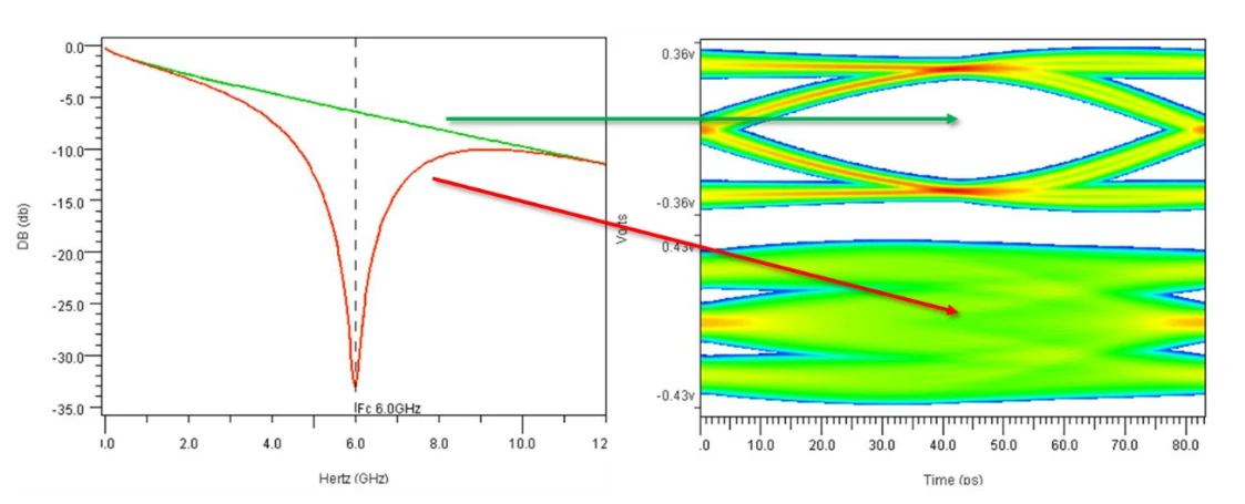
The 250-mil stub causes severe attenuation at the 6 GHz Nyquist frequency, allowing less than 2% of the signal energy to reach the receiver and causing the eye diagram to close completely. Conversely, the 25-mil stub introduces no observable change in insertion loss, yielding a wide-open eye diagram. The longer stub also degrades adjacent frequencies, nearly doubling the channel loss at 5 GHz. Following the presented design guidelines is a practical safeguard against stub-induced resonances that might otherwise noticeably erode the interconnect's performance.

When applying Bogatin’s rule of thumb to modern high-speed links like 112G PAM4, designers must substitute the raw bit rate with the symbol rate (baud rate). Because PAM4 transmits two bits per symbol, a 112 Gbps link operates at a symbol rate of 56 GBd, meaning the physical transitions and spectral harmonics scale from this lower frequency. Plugging 56 GBd into the formula yields a maximum stub length of just 5.3 mils (0.0053 inches). This result aligns closely with the 6-mil maximum stub length calculated using the 7th harmonic criterion, showing how both independent methods converge on nearly identical physical limits for ultra-high-speed channel design.

Hidden Stubs in High-Speed Layouts

As data rates push past 30 Gbps, Bogatin's rule shrinks the maximum safe stub length to a mere 10 mils, roughly the thickness of three sheets of standard office paper. Historically considered microscopic and negligible, a 10-mil feature is now known to be a critical threshold for acceptable channel performance.

At 30 Gbps, the margin for error is so small that tiny metal protrusions off the main signal path can behave like parasitic stubs, requiring engineers to micromanage the geometry of the entire board. Figure 5 highlights how routine layout features introduce these parasitic effects at high data rates, while demonstrating the layout strategies needed to eliminate them.

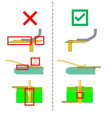
The top item in Figure 5 shows a critical example of a hidden discontinuity that occurs right at the connector landing pad. If a trace is routed into the pad from the wrong side (the end opposite where the connector leg exits), the signal splits at the junction. This routing mistake turns the remaining length of the pad into an unintended stub. In some connector footprints, the landing pad itself can be on the order of 50 mils or more, which is physically long enough to degrade the signal at data rates exceeding 6 Gbps. To avoid this, layout guidelines should mandate point-of-exit routing, ensuring traces always enter from the exact side where the connector pin leaves the pad.

The second item in Figure 5 highlights the hidden stub created by edge-finger connector wipes. When a high-speed plug-in card (such as a Peripheral Component Interconnect Express [PCIe] card) mates with a motherboard slot, the connector pin slides along the gold finger and settles at its final wipe position. This leaves the remaining copper extending to the tip of the finger as an open-circuited stub. While connector manufacturers and industry specifications set this stub length, layout engineers bear the consequences of the resulting signal degradation. At 30+ Gbps, designers can no longer blindly rely on standard footprint libraries; they must actively audit these features and select connectors and finger geometries that minimize the unterminated copper left behind.

The final item at the bottom of Figure 5 highlights the hidden stub introduced by press-fit connector pins. When a press-fit connector is inserted into a plated through-hole, its physical metal pin extends deep into the PCB. As the figure suggests, this issue can be mitigated if the layout engineer routes the breakout trace on the exact opposite layer of the board, utilizing the full length of the pin as the transmission path. However, when signals are forced onto upper or middle layers, the remainder of that metal pin acts as an unterminated stub. To remedy this, 25+ Gbps standards have forced a major industry shift toward surface-mount (SMT) connectors.

Dealing with Via Stubs: Back Drilling

Having established how stubs degrade high-speed channels, the natural next question is how to deal with via stubs, which brings us to back drilling. Back drilling (also written backdrilling) is a fabrication step that re-drills the via from the opposite side to strip away the unused barrel past the target routing layer. Although it adds manufacturing cost and imposes its own design rules on pad sizes and clearances, this process has become the standard method for bringing stub lengths down to the roughly 5 to 10 mil range that modern 30+ Gbps channels demand. Part 2 of this series will examine back drilling in detail: how depth is specified, what layout constraints it introduces, and where it sits among alternatives such as blind and buried vias within high-density interconnect (HDI) structures.

Conclusion

Via stubs are a primary source of signal degradation in high-speed channels, producing resonant nulls and eye closure that worsen as data rates climb. The two rules of thumb discussed here provide a practical first-order check on allowable stub length. It’s also important to remember that not all stubs appear in the via barrel; pads and connector features can harbor their own hidden stubs. These considerations establish both the limits stubs impose and the need for fabrication-level remedies. Part 2 of this series will focus on back drilling, detailing its depth specifications, layout constraints, and how it compares to high-density interconnect (HDI) alternatives.

Related Reading

Part 1: Via Stubs in PCB Design: Resonance, Insertion Loss Nulls, and Back Drilling (this article)

Part 2: Back drilling depth, layout constraints, and HDI alternatives (coming next)

Understanding Fiber Weave Effect: From Glass Weave to Differential Skew by Dr. Steve Arar

Should You Avoid 90-Degree Corners in PCB Traces? by Dr. Eric Bogatin

Quilter PCB Glossary: Back Drilling, Plated Through Hole (PTH), Gold Fingers, and High-Speed PCB Design

Frequently Asked Questions

What Is a Via Stub, and How Does It Cause Resonant Nulls in the Insertion Loss Curve?

A via stub is the unused portion of a via barrel that extends past the target layer where the signal transitions to a routing trace. Electrically, it behaves as an open-circuited transmission line: signal energy coupled into the stub travels to its open end, reflects, and returns to the main signal path. At the frequency where the stub's electrical length equals a quarter-wavelength (λ/4), the round-trip path is a half-wavelength (λ/2), so the reflected wave returns exactly 180° out of phase with the incident signal. This destructive interference creates sharp resonant nulls in the insertion-loss curve and closes the eye diagram.

How Do You Calculate the Maximum Allowable Via Stub Length for High-Speed Designs?

Engineers commonly rely on two rules of thumb to determine the maximum allowable stub length before significant signal degradation occurs. The first is the 7th harmonic criterion, which places the first resonant null at or above the 7th harmonic of the Nyquist frequency, keeping the digital signal's critical frequencies unaffected. The second is Bogatin's rule of thumb, a popular guideline stating that the maximum stub length in inches should be less than 0.3 divided by the data rate in Gbps to avoid severe distortion. These rules let designers quickly estimate safe physical boundaries for high-speed channels before committing to dense simulations.

Which Layer Transitions Create the Longest Via Stubs?

The longest stubs come from transitions that use only a short section of the via barrel, such as a signal that enters on the top layer and leaves on layer 3 of a thick board. A plated through-hole via runs the full thickness of the board, so everything below the exit layer becomes an open-circuited stub. A longer stub resonates at a lower frequency (Equation 4). In the example above, a 100-mil stub with an effective Dk of 6.16 produces a resonant null at about 11.9 GHz, while the 270-mil backplane stub in Figure 3 produces its first null at about 4.4 GHz, close enough to the 5 GHz Nyquist frequency to close the eye of a 10 Gbps NRZ signal.

What Are "Hidden Stubs" in a PCB Layout, and Why Are They a Problem?

Hidden stubs are unintentional stub structures created by routine layout features rather than explicit via barrels. Common examples include surface-mount component pads, connector edge-finger wipes, and press-fit connector pins. These geometries are problematic because they behave like transmission-line stubs: at high data rates, their parasitic capacitance and physical length create unexpected impedance discontinuities and resonant nulls that degrade signal integrity, even when the signal vias themselves are perfectly optimized.

How Does Back Drilling Solve the Via Stub Problem?

Back drilling is a mechanical fabrication step that removes the unused copper barrel of a via. By drilling out this unterminated stub, it pushes the resonant null to a much higher frequency, restoring smooth, monotonic insertion loss rolloff and opening up the eye diagram. While back drilling adds fabrication steps and manufacturing cost, it is a necessary solution for reclaiming signal margin in high-speed digital channels.

Is Back Drilling an Alternative to Blind and Buried Vias?

Yes. Back drilling starts from a standard plated through-hole via and removes the unused barrel past the target routing layer by re-drilling the via from the opposite side. Blind and buried vias within high-density interconnect (HDI) structures are the main alternatives. Back drilling adds manufacturing cost and imposes its own design rules on pad sizes and clearances, but it has become the standard method for bringing stub lengths down to the 5 to 10 mil range that 30+ Gbps channels demand. Part 2 of this series compares back drilling with blind and buried vias in detail.

Does Every High-Speed Via Need Back Drilling?

Not necessarily. A stub needs to be removed only when it is longer than the target data rate allows, and the two rules of thumb in this article give a first-order check. For a 12 Gbps NRZ link, Bogatin’s rule allows a stub of up to 25 mils, and Figure 4 shows that a 25-mil stub introduces no observable change in insertion loss. For a 112G PAM4 link, the 7th harmonic criterion and Bogatin’s rule both put the limit at roughly 5 to 6 mils, which pushes advanced PCB fabrication to its physical limits.

References

Polar Instruments. n.d. "Signal Integrity Effects of Vias, Stubs and Minimizing Their Visibility." Application Note AP8166. Accessed October 26, 2026. https://www.polarinstruments.com/support/si/AP8166.html.

Simonovich, Bert. 2017. "Via Stubs Demystified." Bert Simonovich's Design Notes (blog). March 8, 2017. https://blog.lamsimenterprises.com/2017/03/08/via-stubs-demystified/.

Bogatin, Eric. 2014a. "What is the Bandwidth of a High Speed Serial-Link Signal?: Rule of Thumb #11." EDN. May 7, 2014. https://www.edn.com/what-is-the-bandwidth-of-a-high-speed-serial-link-signal-rule-of-thumb-11/.

Bogatin, Eric. 2014b. "How Long a Stub Is Too Long?: Rule of Thumb #18." EDN. October 23, 2014. https://www.edn.com/how-long-a-stub-is-too-long-rule-of-thumb-18/.

Telian, Donald. 2023. "Fixing the Problem of Stubs." Signal Integrity Journal. January 10, 2023. https://www.signalintegrityjournal.com/articles/2962-fixing-the-problem-of-stubs.