Trick Question: Does a Signal's Rise Time Increase as It Travels Through a Cable?

Why Signal Integrity Is Often Learned on the Job

Signal integrity is not taught at many universities. When the properties of transmission lines are taught, it is usually from an RF perspective, describing the input impedance of a transmission line in the frequency domain. While this is a perfectly fine perspective, it doesn't help a signal integrity engineer understand the time-domain perspective of signal propagation in interconnects.

This means many engineers learn signal integrity on the job. They watch YouTube videos, watch webinars, or learn by doing in the lab alongside more experienced engineers.

Without a solid foundation in the principles of signal integrity, it is easy to misinterpret measurements or simulations and draw the wrong conclusions, screwing up your intuition. I hear too often from engineers that they don't believe simulations, only measurements. These make the perfect audience for me to trick.

A Signal Integrity Teaser Demo

When I present tutorials in front of a large audience of engineers at conferences or on-site at companies, I like to test their understanding with a simple live experiment.

Every oscilloscope has a probe compensation signal used with 10x probes: a 1 V, 1 kHz square wave with a relatively short rise time. Using a small mini grabber-to-BNC adapter, we can measure this signal directly on a scope channel. The figure below shows this setup and the scope measurement of the signal from the short mini grabber connection.

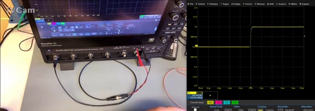
In this example, the 10-90% rise time of the compensation signal is measured as about 203 nsec and the cable is about 3 feet long.

The simple question I ask is: what happens to this rise time if I increase the length of the coax cable connecting channel 1 of the scope to the compensation signal?

I like this example because anyone with a scope and a few coax cables lying around can perform this experiment. I think engineers have tried this measurement or discussed it with others, because every engineer I ask has an opinion. I see too many forums such as Electrical Engineering Stack Exchange, EEVblog, All About Circuits, or RF Electronics where this sort of question is discussed, and too many very misleading answers.

The vast majority of engineers I ask what to expect in this experiment answer that the rise time will increase. The really cool thing about science and engineering is that it is not about opinion; it is about evidence.

When I perform this experiment, adding a length of coax cable, I demonstrate that the rise time does, in fact, increase. In the figure below, I made the cable a total of 12 feet long, and the rise time is 600 nsec, quite a large increase.

In fact, as we increase the length of the coax cable, the rise time will increase at a steady rate. The rise time from three different length coax cables is compared in the figure below. This observation clearly supports the widely held belief that increasing cable length increases the signal's rise time.

This is one of those experiments you should try at home to convince yourself of this behavior.

It is a startling effect. With a length of 6 feet, the rise time is 250 nsec. With 18 feet, the rise time is almost 1 µsec. Does this mean that longer interconnects will cause a significant rise time? If this is true, then how is it possible to transmit a 200 psec rise time 5 Gbps USB signal down a 6 ft USB cable if the rise time will be degraded to 250 nsec, 1000x what enters the USB cable?

Finding the Root Cause: Five Common Explanations

To fix a problem, we need to know the root cause and solve the problem at the root cause. When I ask why this effect happens, I get five common answers:

1. It is rise time degradation from dielectric loss in the cable.
2. It is rise time degradation from conductor loss in the cable.
3. It is the frequency-dependent speed in the cable that causes dispersion and spreading out of the rising edge.
4. It is the signal having to charge up the capacitance of the cable.
5. The signal has farther to travel in the longer cable, and this rise time is related to the time of flight through the cable.

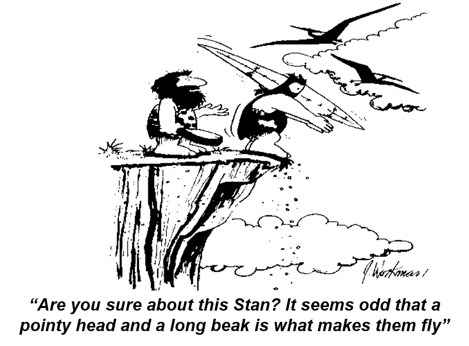
If we have the wrong root cause for a problem, the chance of fixing the problem is based on pure luck. This is illustrated in the cartoon below.

None of the five popular explanations are correct. Relying on any of them to fix this problem is a waste of time. Frequency-dependent losses and dispersion do increase signal time as they propagate on interconnects. However, these effects would impact the rise time about 4 orders of magnitude less than what is observed.

If cable capacitance causes the longer rise time, then you would shorten the rise time by using a lower-capacitance cable. This won't work either. The last explanation is just meaningless. There is nothing to act on.

The real reason the measured rise time increases with cable length has to do with how signals interact with the complete system composed of the transmitter (TX), the interconnect, and the receiver (RX).

The Real Explanation: An Equivalent Circuit Model of the System

To understand a real-world system, we have to translate it into an ideal equivalent circuit model. This process is called situational awareness.

Once we have the ideal circuit model, we can apply our foundational principles to predict signal behavior. We compare the predicted signal behaviors in the virtual world with the measured behaviors in the real world. We try every consistency test we can in the virtual ideal world and look for the same predicted behaviors in the real system.

I am not sure if we can know for sure if we have a correct explanation, but the more consistency tests we do, with a correlation between the simulated behaviors of the signals and the real measured behaviors, the more confidence we have that we are closer to the truth.

The complete equivalent circuit model of this measured system is shown below.

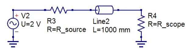
The simple first-order model of all signal sources is a Thevenin equivalent. It has an ideal voltage source, a step edge with a voltage and rise time, followed by a source resistance. Surprisingly, many IBIS (Input/Output Buffer Information Specification) driver models match this simple model very well.

The cables of various lengths are modeled as ideal uniform, lossless transmission lines. They have just two attributes: a time delay and a characteristic impedance. The scope channel, the RX, can be modeled as a simple ideal resistor.

With this model, we can understand all the effects we see with the comp signal, different-length cables, and even the two different scope input impedances: 1 megohm and 50 ohms. To use this model, we need to know the attributes of each component.

Characterizing the Probe Compensation Signal

Understanding the Thevenin output resistance of the comp signal, and the signal's properties on transmission lines, is key to understanding why the measured rise time increases with cable length.

To measure the Thevenin output voltage of the comp signal, measure the "open circuit" voltage with the scope. This means keeping the scope on the 1-megohm input and waiting for all reflections to die down to see the steady-state voltage. If the cable is 3 ft long, the time delay is about 6 nsec. One cycle of ringing would last 4 time delays or 24 nsec. If we wait 40 ringing cycles, this is 1 µsec, plenty of time for the steady state. The figure below shows the measured voltage on the scope with a 1-megohm input impedance.

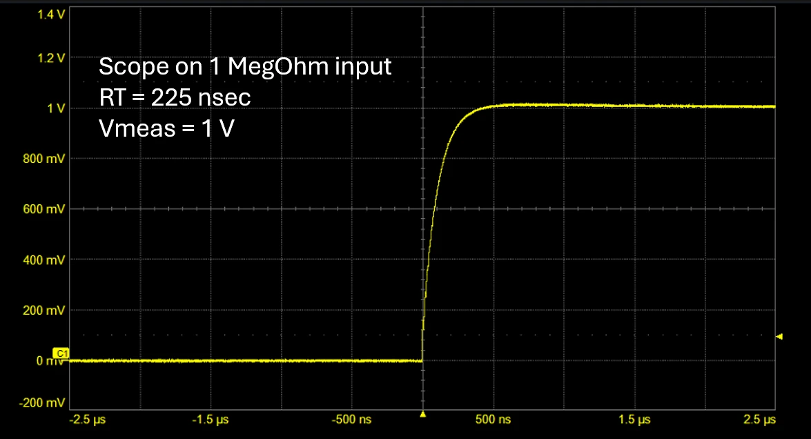
The Thevenin voltage is 1 V. To get the Thevenin resistance, we add a known load to the driver and measure the change in voltage across the load. The change in voltage is literally the voltage across the Thevenin resistance. The current through the Thevenin resistor is the voltage across the load resistor.

When we connect the 50-ohm resistor of the scope across the source, we will see the output of the source drop because of the voltage divider we created. From this measured voltage, we can calculate the Thevenin resistance of the source. This measurement and analysis are shown below:

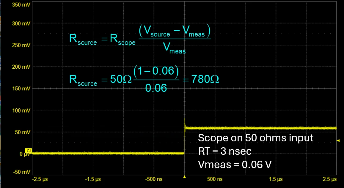
We predict the loaded voltage to drop from 1 V. The measured voltage of 60 mV means the Thevenin source resistance of the comp signal is about 780 ohms. This is critically important. Why is it so high? I asked some of my scope designer buddies, and they say the exact value is not important, as long as it is high enough so that if the scope user accidentally connects the 10x probe ground lead to the comp signal output, the current through the ground lead is very small.

I know none of my readers would ever do that, but I see many of my students not paying attention to the labels and connecting the 10x scope probe's ground lead to the signal lug all the time. It's a good thing the comp signal output impedance is high.

We get a two-for-one measurement in this test. If we set the scope to 50 ohms, there are no reflections when the signal moves from the 50-ohm cable to the 50-ohm scope input impedance, and the signal we measure by the scope is the signal launched into the 50-ohm coax cable. What the scope measures is the signal directly out of the comp signal. This signal has a rise time of 3 nsec. Now we have the three important attributes of the comp signal. Its Thevenin voltage is 1 V, its Thevenin resistance is 780 ohms, and its rise time is 3 nsec.

This test also demonstrates so clearly that if we use a 50-ohm input to the scope to prevent multiple reflections in the cable transmission line, the actual rise time we measure, independent of the cable length, is actually 3 nsec. This is the intrinsic rise time of the comp signal, not the nearly 1 µsec we measured with an 18 ft cable and 1-megohm input of the scope.

Table 1: Measured Rise Time of the Probe Compensation Signal by Cable Length and Scope Input

But why do we see the longer rise time? This is where analyzing the signal's interaction with the system step by step matters.

How Reflections Stretch the Measured Rise Time

It all comes back to the system model. When the 1 V signal from the source goes through the 780-ohm source resistor, it sees the initial input resistance of the transmission line of 50 ohms. This makes a voltage divider with the Thevenin source resistance. The voltage launched into the transmission line will be:

1 V × 50 ohms / (50 ohms + 780 ohms) = 60 mV

This 60 mV signal will propagate down the transmission line to the 1-megohm input of the scope. It will reflect with a reflection coefficient of nearly 1. The scope will measure the incident 60 mV signal + the reflected 60 mV signal. The scope can't tell the direction of propagation of a signal, only the total voltage of the signal. This means 1 time delay after the 60 mV signal enters the coax cable, the scope will measure a signal of 120 mV.

The 60 mV reflected signal will travel back to the source. When the 60 mV signal hits the 780-ohm impedance of the source, it will reflect with a reflection coefficient of about 0.9. About 54 mV will reflect back to the scope input. When the 54 mV signal hits the 1-megohm input of the scope, another 54 mV will reflect. The scope will see the previous 120 mV, and the new 54 mV + 54 mV = 228 mV.

If the coax cable is 12 feet long, its time delay will be about 25 nsec. The round trip from the scope to the source and back will take 2 time delays, or about 50 nsec. We should see steps in the received signal at the scope with a duration of about 50 nsec. The initial step will be 120 mV and a second step, 50 nsec later of 228 mV.

This is precisely what is measured, as shown in the figure below.

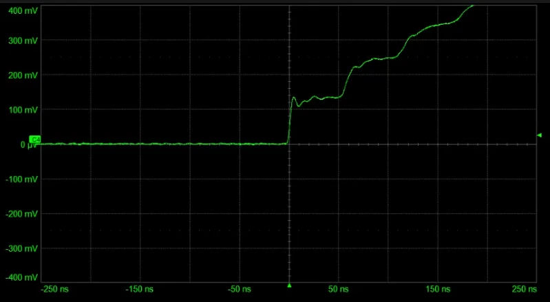
Each step is 50 nsec long; each step diminishes slightly with each reflection from the 780-ohm impedance of the source. This is an exponential behavior. It looks like an RC time constant, but it has nothing to do with an RC charging. It has to do with a small initial voltage launched into a transmission line and the reflections back and forth between the high-impedance source and the high-impedance scope.

As the cable length increases, each step in the staircase up to the full Thevenin voltage lengthens, and the rise time increases. Does the rise time actually increase with increasing cable length? In this specific system, absolutely. Anyone can measure this. But there is a difference between the source's intrinsic rise time and what the scope actually measures. The system matters.

If this is the root cause, how do we reduce the rise time through an interconnect? The root cause is the reflections from the 1 megohm of the scope and the 780 ohms of the source. This causes the signal to bounce back and forth, increasing the apparent rise time.

The solution is to use a termination strategy at either end to prevent the signal from rattling around. We saw this in the example above when we used a scope impedance of 50 ohms. This prevented reflections from the coax cable and the scope input. The signal we saw on the scope was the signal launched into the coax cable, with the source's rise time. We had such a small voltage launched into the transmission line because the source impedance was so high.

If we want a larger signal measured by the scope, we need a lower output impedance source.

Two Final Puzzles

If you have never studied the properties of transmission lines except in the frequency domain, the behavior of signals on transmission lines can sometimes seem counterintuitive.

To test your understanding of transmission lines, consider these two simple puzzles.

Puzzle 1: Ringing with a Low-Impedance Source

Remember the signal the RX sees is not about the source. It is about the system composed of the TX, the interconnect, and the RX. Suppose the source impedance is very low, much smaller than the transmission line characteristic impedance. And we set the scope impedance to be 1 megohm. What do we expect to see as the signal into the scope? I will tease you with the answer, as this is the poster child for signal integrity behaviors. Here is the measured signal as seen by the scope in this case.

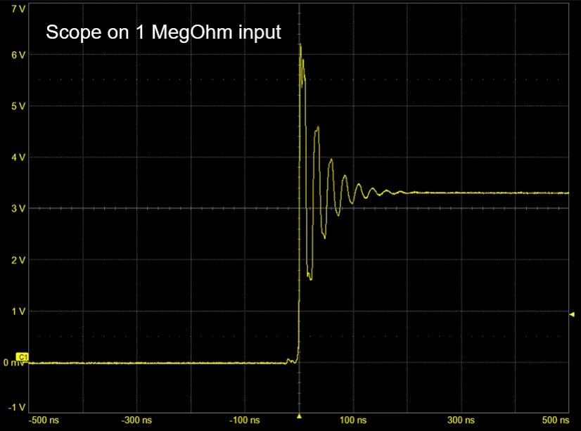
Why is there ringing, and what can you do in the system design to reduce this ringing, based on the root cause?

Puzzle 2: An Ohmmeter on an Earth-to-Moon Coax Cable

The second puzzle will test your understanding of transmission lines and the difference between instantaneous impedance and characteristic impedance.

Suppose we have a very loooong 50-ohm coax cable. In fact, it is so long, it stretches between the Earth and the Moon. It is open at the far end on the Moon. If we connect a simple digital multimeter (DMM) as an ohmmeter between the signal and return connectors at the front of the cable, what resistance will the ohmmeter read? This is illustrated below.

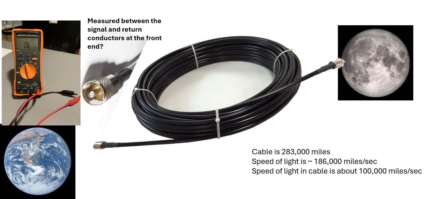
Let me qualify this. What will the ohmmeter measure in the first 1 second, the first 5 seconds, and after 1 day of being connected? If you understand transmission-line principles, as every engineer designing boards with signal rise times shorter than about 10 nsec should, this is a no-brainer.

Transmission Line References

If you want a refresher about transmission lines, check out these three references:

• My textbook, Signal and Power Integrity: Simplified
• My textbook, Practical Guide to Transmission Line Design and Characterization for Signal Integrity Applications, with the accompanying free videos
• My free video master class on transmission lines

Conclusion

Transmission line properties and signal behavior on transmission lines are foundational to signal integrity. The design process is creative and relies on engineering intuition. Without a clear intuitive understanding of transmission lines, you will be trapped by blindly using design guidelines where they may not apply.

Investing time in understanding how transmission lines behave in a system is well worth it. It will give you a completely different perspective on how signals interact with systems.

Frequently Asked Questions

Does Cable Length Increase a Signal's Rise Time?

The rise time you measure can increase with cable length, depending on the rest of the system. In the oscilloscope experiment in this article, the measured 10-90% rise time of the probe compensation signal grew from about 203 nsec with a 3-foot coax cable to about 600 nsec with 12 feet and almost 1 µsec with 18 feet. The cause was reflections between the high-impedance source and the high-impedance scope input. Frequency-dependent loss and dispersion also degrade rise time as a signal propagates, but in this setup their effect was about four orders of magnitude smaller than what the scope showed. With the scope input set to 50 ohms, the measured rise time was 3 nsec at any cable length.

What Changes When You Switch an Oscilloscope from a 1-Megohm to a 50-Ohm Input?

With a 1-megohm input, a signal arriving on 50-ohm coax reflects with a reflection coefficient of nearly 1, and the scope displays the sum of the incident and reflected signals. If the source impedance is also high, the signal bounces back and forth in the cable and the measured edge becomes a staircase. With a 50-ohm input, the scope terminates the 50-ohm cable, so there are no reflections, and the scope shows the signal launched into the cable with the source's own rise time. For the probe compensation signal in this article, that was 3 nsec, at an amplitude of only 60 mV, because the 780-ohm source and the 50-ohm load form a voltage divider.

How Do You Measure a Source's Thevenin Resistance with an Oscilloscope?

Measure the open-circuit voltage with the scope on its 1-megohm input, and wait for reflections to die down so you see the steady-state value. That is the Thevenin voltage. Then load the source with a known resistance, such as the scope's 50-ohm input, and measure the loaded voltage. The source and load form a voltage divider, so R_source = R_load × (V_open − V_loaded) / V_loaded. For the probe compensation signal, 50 ohms × (1 V − 0.06 V) / 0.06 V gives about 780 ohms.

Why Does an Oscilloscope's Probe Compensation Output Have Such a High Impedance?

According to the scope designers quoted in this article, the exact value is not important as long as it is high enough that, if a user accidentally connects the 10x probe's ground lead to the compensation signal output, the current through the ground lead is very small. On the scope in this article, the Thevenin source resistance of the compensation signal measured about 780 ohms.

How Does Termination Fix the Longer Measured Rise Time?

The longer rise time comes from reflections at both ends of the cable: the 780-ohm source and the 1-megohm scope input. Terminating either end stops the signal from bouncing back and forth. In the experiment in this article, setting the scope input to 50 ohms terminated the cable at the receiver, and the scope showed the source's 3 nsec rise time. Because the source impedance was so high, the terminated signal was only 60 mV. A larger signal at the scope would require a source with a lower output impedance.

When Do You Need to Think About Transmission Lines in PCB Design?

The threshold in this article is rise time: every engineer designing boards with signal rise times shorter than about 10 nsec should understand transmission-line principles, including how signals behave in the time domain. In the model used here, an ideal lossless transmission line has two attributes, a time delay and a characteristic impedance, and the signal at the receiver depends on the whole system: the transmitter, the interconnect, and the receiver.

Should You Trust Simulation or Measurement in Signal Integrity?

The method in this article uses both. Translate the real system into an ideal equivalent circuit model, apply foundational principles to predict signal behavior, and compare the predictions with measurements. Each consistency test that agrees adds confidence that the explanation is close to the truth. In this article, a model of a 780-ohm Thevenin source, a lossless 50-ohm cable, and a 1-megohm scope input predicted a first step of 120 mV at the scope and a second step of 228 mV about 50 nsec later on a 12-foot cable, and the measurement matched.

Sources

Bogatin, Eric. Practical Guide to Transmission Line Design and Characterization for Signal Integrity Applications. Artech House, 2020. Companion videos at Signal Integrity Journal, April 1, 2024. https://www.signalintegrityjournal.com/articles/3526-sij-university.

Bogatin, Eric. Signal and Power Integrity: Simplified. 3rd ed. Pearson, 2018. https://www.amazon.com/Signal-Power-Integrity-Simplified-Prentice/dp/013451341X.

Bogatin, Eric. "Should You Avoid 90-Degree Corners in PCB Traces?" Improving the Signal-to-Noise Ratio, Quilter, October 8, 2026. https://www.quilter.ai/blog/90-degree-corners-pcb-traces.

The EEcosystem. "Masterclasses." Accessed November 5, 2026. https://www.theeecosystem.com/masterclass.

Related Reading

• Should You Avoid 90-Degree Corners in PCB Traces? (Improving the Signal-to-Noise Ratio, Part 1)
• Stephen Newberry and the Discipline of Signal Integrity
• Via Stubs in PCB Design: Resonance, Insertion Loss Nulls, and Back Drilling (Via Stubs and Back Drilling, Part 1)

About Dr. Eric Bogatin

Dr. Eric Bogatin is Technical Fellow at Quilter, the Physics-Driven AI platform for PCB Layout Automation, and advises its physics and engineering teams. He is a professor in the Department of Electrical, Computer, and Energy Engineering (ECEE) at the University of Colorado Boulder, where he teaches graduate-level signal integrity courses and the Senior Design Lab Capstone Course. He is the former technical editor of Signal Integrity Journal, a Fellow with Teledyne LeCroy, and the Dean of the Teledyne LeCroy Signal Integrity Academy. He is the author of 18 books on signal integrity and electronics, including Signal and Power Integrity: Simplified (Pearson, 3rd edition, 2018), Principles of Power Integrity for PDN Design: Simplified (2017), and Practical Guide to Transmission Line Design and Characterization for Signal Integrity Applications (2020). He holds a B.S. in physics from MIT and an M.S. and Ph.D. in physics from the University of Arizona.